May 5th, the little things in life
In which I conclude my own ad hoc quest for patterns and recount adventures slicing up sunflower and cucumber stems.
It is raining, solidly, casting a pall over Laura’s and my plans to be good cultural tourists and tour some National Trust sites round about (to wit, Felley Priory and Newstead Abbey). The UK Met-Office weather map shows storms all suddenly exiting stage right (watch out Skegness!) but just in case they call this one correctly, I am blogging over breakfast to avoid having to write later in an exhausted heap having set foot on every square inch of Priory and Abbey.
Because I rather ‘copped out’ in last week’s post (although do have a look at the scary photo if you missed it), I have two weeks worth of exploits to recount here, not only a larger than usual chunk of time but also both of my projects were in play. So this will probably be yet another longwinded post. Grab your coffees!
If there are any readers sufficiently dogged or idle to have made it to the end of the April 19th post, they will have seen the “Pattern” plot and the “New Data” plot. [to be fair, I didn’t name them then but I have gone back and named them now.] The Pattern Plot found a pattern in the swarms of root velocity curves with respect to time, and the New Data plot was a set of new data with which I hoped to check for repetition. Well, here is the same analysis that produced the Pattern Plot but applied to the new data set:
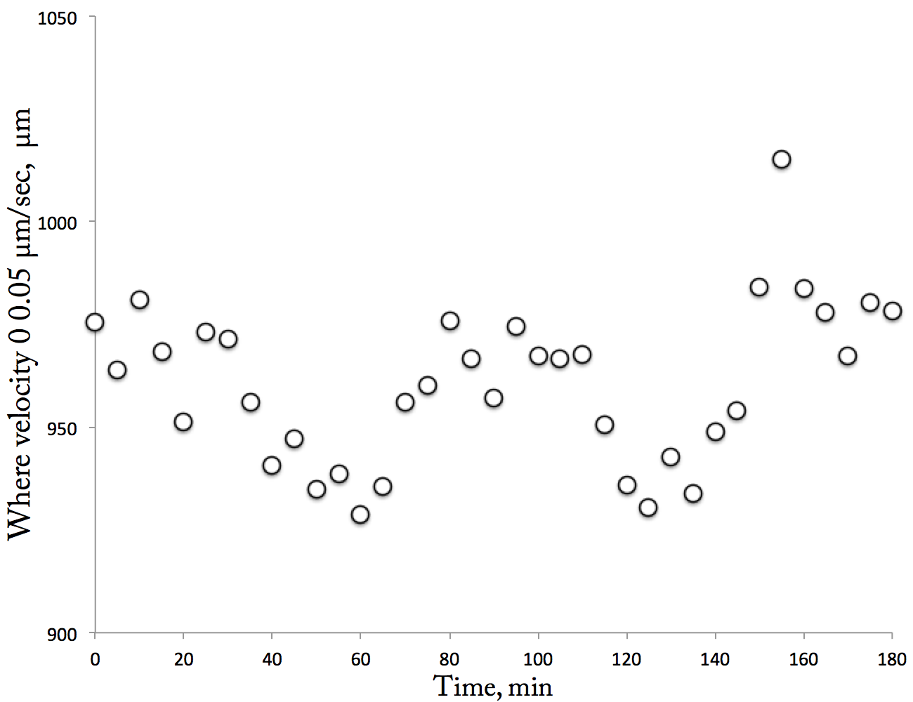
The Repeated Pattern plot. The position where velocity = 0.05 µm/sec plotted as a function of time. Each datum represents a single velocity profile. The position was obtained from the best-fit line through the points between 800 to 1100 µm.
Oh ho! Now that looks like a pattern. To remind you, this analyzes the elongation zone and plots the position where a specific value of velocity is reached. That value (0.05 µm/sec) is in the middle of that zone and is calculated by fitting a linear regression line to the data between 800 and 1100 µm. The happy little sine wave in the Repeated Pattern plot implies that the position of the transition to rapid elongation moves back and forth in a regular way. And to get really fancy and make comparisons, note that the original Pattern plot goes over 90 min whereas this one goes over 180 and so the time scale of the pattern in each is reasonably similar.
Well this repetition strikes a blow against noise. But still. I realized that I am making all of this analysis up. I need to talk with someone who analyzes noise in data for a living: that is, a statistician. The linear regression trick seems arbitrary and ad hoc. I’d like to see how these curves can be analyzed more rigorously for time dependent changes. In the meantime, I have made and will keep making more movies. Analysis can happen anytime, even back home in USA, but making movies requires the laboratory and the better part of a day (as well as the time to plate seeds and grow them).
While questing after root velocity patterns, I did not forget my segments. Again, long term readers will recall my frustration with the maize mesocotyl, half of whose segments responded to auxin with alacrity and the other half sluggishly or not at all. I decided I would see other plants, specifically sunflower, cucumber, and pea. I chose them because they are all good looking but also because they have been used more or less frequently in the history of stem growth research. So far, I have done experiments with sunflower and cucumber. I use the seedling stem, which in these plants is called a hypocotyl. This organ is functionally similar to the maize mesocotyl but rejoices in a different word because botanists. (Sorry – cheap crack—there are real anatomical differences between grass seedlings and those of non-grass seed plants, so the terminology has a point).
Here are the results. Note that all of the numbers in these tables give growth rate in units of % per hour. In all cases, the auxin concentration was 10 µM and the acid pH was 4.0.
… Sunflower Table
….elongation rate widening rate
… Auxin acid Auxin acid
Dish 1 5.2 1.8 0.7 1
Dish 2 5.4 3.4 0.3 0.2
Dish 3 6.4 1.3 0.1 -0.8
…. Cucumber Table 1
….elongation rate widening rate
Auxin acid Auxin acid
Dish 1 4.3 2.9 -1.0 -1.0
Dish 2 5.0 4.1 -0.8 0.3
Dish 3 4.7 4.1 0.4 0.9
…. Cucumber Table 2
….elongation rate widening rate
Auxin acid Auxin acid
Dish 1 3.1 3.1 0.7 0.8
Dish 2 3.7 3.8 -0.4 -0.3
Dish 3 4.3 3.5 -0.1 0.3
Wow! A lot of numbers. The point of all of this was to ‘get the feel’ for using these various species and see which one might prove to be best for further use. Unseen here are the observations that the sunflowers germinate quite irregularly, meaning that I have to plant a bunch to get a set of stems of about the same length for experiments. In contrast, the cucumbers are beautifully regular. However they grow more slowly in the box and are more difficult to cut. Well, a disclaimer on the last point – maybe my blades are getting dull? After that last experiment, I changed them.
But the numbers also show things. First, and perhaps most important, none of them did that Jekyll and Hyde thing that the maize stems did. The variation in the dishes was continuous and not too enormous. The sunflower responded more vigorously to auxin than the cucumber. That is one reason why I did a second cucumber experiment. This might fit with the cucumber growing more slowly in the box than the sunflower. In contrast, the sunflower seemed to respond more weakly to acid than did the cucumber. But I cannot be definitive about that because the acid for that experiment was 25 mM citrate, whereas for the cucumbers it was 10 mM citrate. It is possible that 25 mM citrate is too high, in the same way that 50 mM sucrose caused substantial growth inhibition (in an earlier maize trial).
As for widening, all the data average up to about zero. It is clear that this method of measurement is not sensitive enough to capture small rates of change. But at least they can rule out any large shrinkage in the acid treatment, although I’ll be more satisfied with this conclusion when there is a stronger elongation response to acid. Nevertheless, and also not seen in the numbers, there is an interesting effect going on. Under auxin, the pipe-like shape of the segments is more or less preserved but under acid, they tend to undulate. This is clear enough that I can tell whether a final image of segments was of an acid or of an auxin treatment. I am not sure what it means and quantifying will be far from trivial.
For this coming week, I planted pea. With those results in hand, I will choose my ‘favorite’ for further experiments. I might need to make more washer dishes so that I can do experiments with 9 dishes, increasing the variables that can handled in one go. Or perhaps I can use 9 segments per dish and get away with two dishes per test? I need to see what the growth rate of segments without any addition is. I need to see if I can get a bigger acid bang, perhaps with just HCl? Checking what happens with gibberellin and kinetin would be useful too. Finally, I am curious whether I can get cationic beads to cling to the stems, making perhaps a more accurate way to measure growth than by using the ends of the segments. Lots to do and suddenly shrinking time to do it in! Don’t panic! Deep breaths…