July 5th – I got rhythm
In which I return to the stable root velocity profile problem and describe the results of a forray into numerical analysis.
It was a short week among the benches. On Tuesday evening, I got back from a two-week holiday, happy but exhausted. It was not one of those lay-on-the-beach-like-a-rutabaga spells but rather a visit-all-sorts-of-friends-and-see-all-sorts-of–things holiday. We did set feet on two beaches, and glorious beaches they were, Rhossili and Ynyslas, both in Wales, but to walk and explore thereon, not to idle away the day slathered in sunscreen and sea salt.
Being thus drained, it was perhaps a providence that the two experiments I had planned for Thursday and Friday went ‘roots up’. Best laid plans and all that. I had planed to make two more movies for the ‘stable root growth project’, and had plated the seed before I left and asked Darren to move the plates from the fridge to the growth chamber the Monday of the previous week. Upon checking this Wednesday, the roots were too small. Upon further checking I found that a light bulb for that rack had burnt out and even more that, while they were stashed in the fridge, the plates had gotten pushed to back and sort of froze, as things some times do at the back of the fridge. The burnt-out light is a plausible explanation for slower than expected root growth, and the freezing would not have helped. I plated another round on Friday and am hoping that the week after next I can take the relevant additional movies. Now is really not the time to suffer random failures of plant growth.
Nevertheless, there is progress to relate. The day before I left for the holiday, there was an event. Drama! Excitement! This too relates to the ‘stable-root-velocity-profile’ project. Back on May 24th (here) I wrote of how I detected a rhythm in the profiles of a root over time but that the analysis I used to see this was ad hoc, and not particularly rigorous. It had become clear to me that doing any sort of rigorous analysis was over my head, way over it, and that I needed help.
I enlisted help, in the form of Simon Preston, of the UofN Maths department. In my first meeting with him, after explaining what I was after and getting his interest, I left him with the two datasets that I had by then produced. To be clear, a dataset comprises 37 or 38 velocity profiles for a single root. The profiles are taken every 5 minutes (the total span is 3 hours). Simon developed a treatment based on principal component analysis. Essentially what this method does is to treat the dataset as an N-dimensional volume and search for axes (termed components) piercing the volume along which the data vary the most. Such an axis captures variation in the data and thus has the power to explain it. But I cannot explain principal component analysis any better than that. Simon wrote a MatLab program that takes the dataset as input, carries out the analysis, and low and behold (!) the first principal component resembles the rhythm I had found more or less by hand. Cool.
But perhaps not entirely convincing with a sample size of two, and one of those was a bit sketchy. Now, to create the input dataset takes a bit of doing—I need to generate 37 or 38 raw velocity profiles from the movie of the growing root. There is a bunch of hacking around on the computer to set it all up. Here is one task—finding the zero point for each of the 37 (or 38) times. Recall that the velocity profiles start at the root tip, easy in concept but what point to use for x = o in practice? Recall further that to have roughly the same sized velocity profile over three hours, while the root is growing at hundreds of microns per hour, I change the position of the root by hand every 5 or 10 minutes, and it is essential that the point I use for the zero point is the same for each time point. One might venture that the very end of the root cap, the last point so to speak on the root, would work, but this point is formed by large and floppy cells and over the course of the 3 hours their shape changes markedly. What I do is to cut and paste images of the tip of the root into a single file and find the best reference point to line them all up (see image below). Thankfully, the arabidopsis root tip contains starch grains that scatter light strongly, making a set of dark bands. Typically the space between these is narrow and relatively constant over the movie.
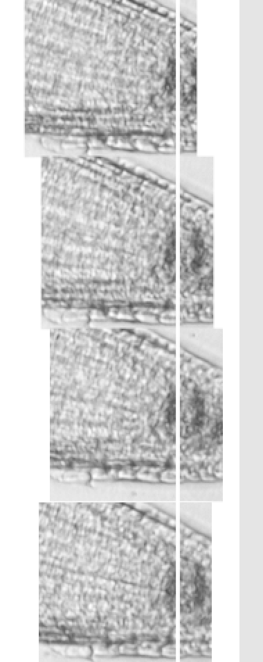
A portion of the set of root tip images used to define a specific point as x = 0. The dark bands are starch grains of the root cap. I use the white line to adjust each tip image and find a common point.
In any case, I happened to have finished making the dataset for a third root just in the few moments of down time between arriving (by train and cycle) and my meeting with Simon for a second round of discussions. I had my computer along and with Simon looking over my shoulder, I fed the new dataset into his program, and out popped this:
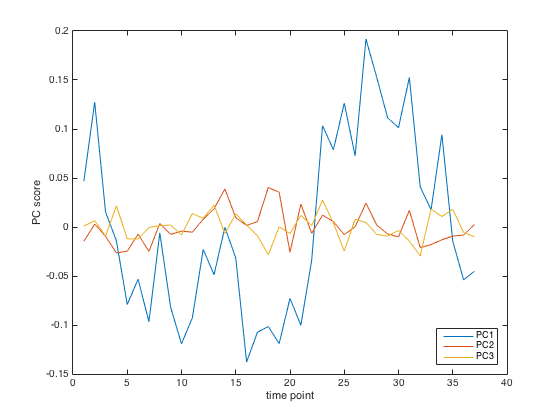
Principal component analysis of April 23 root. The slice through the dataset represented by PC1 (blue) appears to vary rhythmically.
As it did for the previous two roots, principal component 1 (blue line) pulls out a rhythm. Clear as you please. Simon and I, seeing this emerge more or less Venus-like from sea foam, were struck dumb with wonder. Well not exactly, but it was an exciting moment.
To be sure, being able to say that principal component number one really does vary is a long way from saying what that variation represents (disclaimer, while three out of three is looking good, to say that it “really does vary” will require statistical testing, hooray!). Because the variation resembles closely what I was doing by comparing regression lines, I am hopeful that an explanation can be found along those lines (pun intended!). But that is for the future. For now, I got a rhythm! Who could ask for anything more?