April 11th, Back to my roots
I have abandoned the maize mesocotyl. Before getting into all that, here’s a shout out to my son Nick, who blogs about music on Nonstandard Repertoire but chose the other day to post about his favorite enzyme, rubisco. Check it out!
When to stop throwing good money after bad? Now, it seems. Enough mesocotyls! I did a pilot test growing sunflower and cucumber seedlings in the dark boxes to learn what day to harvest them, and this past Friday, I set sunflowers up for an experiment this week. Week before last’s experimental layout was successful – three dishes with auxin, three with acid. I can see how well acid and auxin turn on growth, and above all, test the variability. After that try cucumber and pea, and chose the one that looks the best for further work.
With all this segmental obsession, readers might be surprised to learn that I have not abandoned my root growth project. Yes, the last blog post on my root growth experiments was way back in November (here), but I have been continuing the root growth project, just keeping mum. The segment experiments lend themselves to bloggery quite well: there is one run per week; and with each run, some problem crops up, and so the next run involves a possible fix. One could set it to music. Counterpoint. The root growth experiments? Not so much. They don’t follow a weekly rhythm and they are addressing issues that are difficult even to think about let alone explain. But it is time to have a go.
Before describing the work, I provide background, rather a lot of it. Knowledgeable or impatient readers may skip down to the [#] below.
The heart of the matter is the velocity profile for the root’s growth zone. I have written about this previously (e.g., here), but because the issue is indispensible to what I am trying to do, I am going to start fresh, rather than making you fossick through old posts. Let me start with a picture:
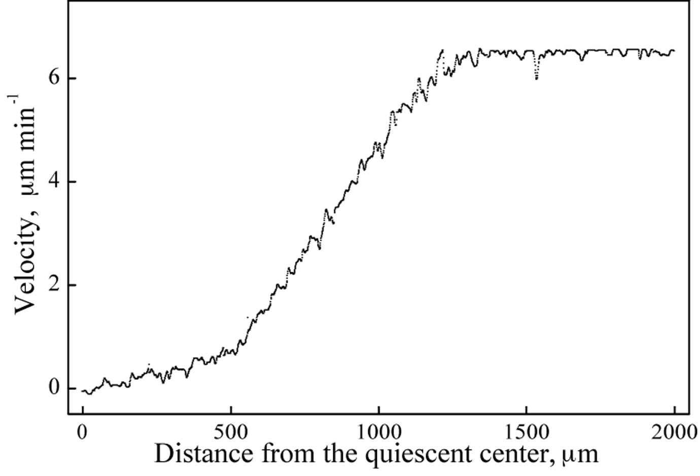
Velocity profile of an arabidopsis root
The x-axis is distance from the quiescent center, but for now take it as distance from the very tip of the root. The y-axis reports velocity, something that should not be surprising for a velocity profile. Let’s start with a straightforward concept: root growth rate. If you were to measure the position of the root tip at defined times, it would move downward through the soil and your measurements would define how fast it was moving, in other words, its velocity. This is what is meant by root growth rate and it is an obviously relevant physiological parameter, testifying to the root’s vigor, acclimation state, and all the rest.
But what makes the root tip move? That motion is caused by cells in the root getting longer. They take up water and increase their volume, mostly in length. Thus, the part of the root behind the tip gets longer (this is growth) and so the tip is moved. The rate of root growth thus integrates the growth of all the cells in the root.
Now, we want to know what each cell is doing, and even what sub-cellular regions are doing. We get this by measuring the velocity of all of the moving parts of the root. Imagine sprinkling a bunch of tiny ink spots all over the root and photographing the root over time as it grew. Spots in the mature, non-growing part of the root would be motionless, there would be no cells elongating to make their position change. An ink spot near the base of the growth zone would move a little bit because there would be a few cells elongating between it and the non-growing (i.e., stationary) part of the root. A spot a bit closer to the tip would move a little faster because there would be a few more cells between it and the non-growing part of the root, and so on, until reaching the tip, which would have the maximal velocity because all of the growing cells are interposed between it and the non-growing part. By measuring the movement of all these spots, one gets the velocity profile.
When comparing that imaginary exercise to the figure above, it seems upside down. In the figure, velocity is zero at the tip and rises to reach a maximum at about 1200 µm from the tip (that maximum is a bit faster than 6 µm per minute). Yes, it is upside down! I have done one of those transformations that mathematicians are always banging on about to make the maths easier. Well that is not a bad thing. In this case, the tip has been apposed to an infinite and immobile surface, forcing it to be motionless (a velocity of zero). This makes growth move material in the opposite direction, that is, towards the mature end. That maximum rate (a bit more than 6 µm/min) plotted at the back end is actually the rate the tip moved (the rate of root growth). This is physiologically silly (stems don’t get pushed up toward the sky) but mathematically essential.
The velocity profile is the integral of local expansion rates. Or to put that another way, the derivative of the velocity profile (the curve in the figure above) represents local (i.e., sub-cellular) elongation rate. This is the major reason why velocity profiles are sought after—their derivative gives the growth action. This is key information for anyone like me who wants to understand the growth process itself.
The profile has distinct regions—from zero to about 500 µm, velocity increases gradually with distance (which means local elongation rate is low in this region), and then the velocity increases steeply with position up to about 1200 µm (and so elongation rate likewise increases, by about tenfold), and finally velocity becomes constant (elongation rate is zero). In other words, the velocity profile has two big kinks, that separate zones of distinct growth rates.
[#]
OK, with that background, I can move into what I am trying to do. The figure above presents the velocity profile at essentially one instant in time (in fact it took a few minutes worth of imaging to acquire). I am interested in understanding how that profile is maintained as the root grows. The way to do this seemed straightforward—image the root over time and look at the sequential velocity profiles. I did so and way back in October posted results like this (maybe even exactly this):
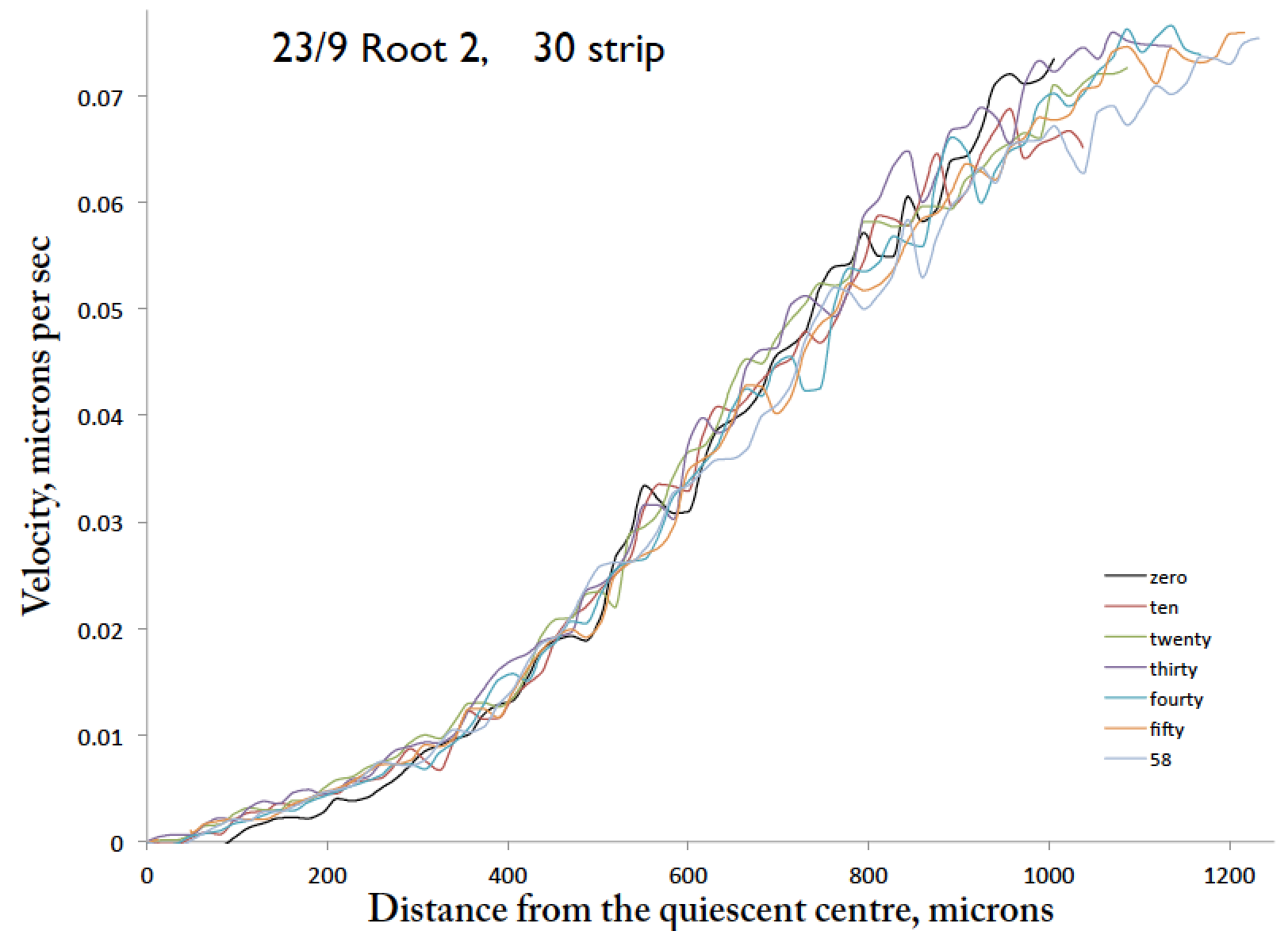
A set of velocity profiles for a root taken at ten minute intervals, with forty spelled wrong in the legend, because English.
This shows the velocity every ten minutes for about an hour. The profile looks pretty stable. But how stable is it? There are wobbles – is this signal or noise? This is just one hour—how about longer intervals? To get the above data, I started the root off about 3/4 of the way across the field and so as time advances there is more and more root in the field, and after one hour the tip has reached the end of the frame. That is why the curves are not all the same length. I’d like to go for a longer time period, but if I start the root off at 1/2 way across the field, then the early profiles are quite a lot shorter, and comparing profiles of notably different lengths bites.
I tried a few runs where I started the root off at 3/4 of the way across, and after an hour, moved it back to the 3/4 position and kept recording. In the several examples I analyzed like this, there was a jump in the velocity profiles when the root was moved back. Maybe, the roots noticed my moving them back up? That would be a biological explanation. But there is also an experimental or systematic possibility. It turns out that before the software can calculate the velocity profile (which it does from a pair of images separated by a mere 60 seconds) I have to specify a few points along the root’s midline. This is because the roots are not plumb lines: they bend. The velocity of interest comes from elongation and one needs to calculate the velocity parallel to the midline. Finding a midline is one of those things that the human eye does really well but computers do really badly. Therefore, a few points along the midline are put on by hand, and the computer draws the midline from these. As the root takes up more and more of the field, the points chosen for the midline have to be a little different. This does not cause a big change in the calculated velocity profile, but it might be enough to cause a little jump in the profiles when the root was re-positioned.
Therefore, I decided to try a different approach: Instead of moving the root in one fell swoop, I would move it incrementally and continually so the root would always span the full field. This did mean that Darren Wells had to rewrite the time-lapse acquisition program so that it would show me the live image in between capturing, but apparently that was straightforward. For these runs, I had to sit by the microscope to adjust the position of the root every five minutes, Tobias the human servo motor, but we all know doing science is boring.
I made several movies like that and found a new problem. Even though on average the root grows straight down the plate, following gravity, in practice it wanders, growing now to the left and now to the right. This means that while I am carefully adjusting the position of the root tip to be at the end of the frame, the root is moving sideways and bending too. So again, sigh, the shape of the midlines alter over the course of imaging. Not only that, the transient growth adjustments shifting the root into these digressions will add a further level of noise to the velocity profiles.
While pondering these issues, serendipity struck. I was quite literally holding the plate of seedlings in my hand staring at them, when I noticed amid all the wanderers, one root growing down the plate as straight as taut violin string. This root had gotten itself inside the agar medium, rather than as usual on the surface. All of this pushing left and right comes down to interactions between the root and the surface of the agar. Put the root inside the agar and all that vanishes and the root grows straight. An aha! moment – I should image roots inside the agar. And I held in my hand a plate with such a root.
The next day I imaged that root, for ninety minutes, moving the plate a touch between each pair of images, taken at five min intervals. Here is what I got:
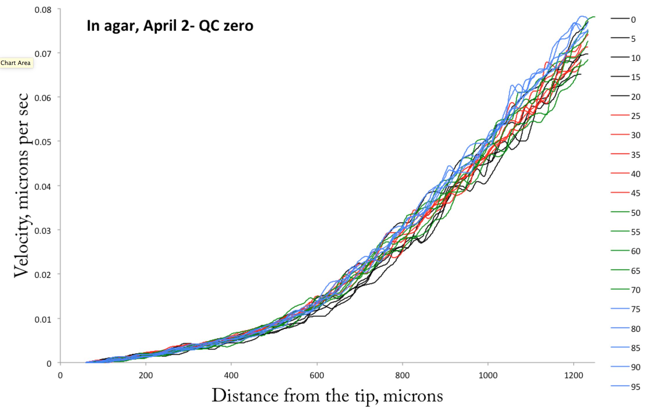
A set of velocity profiles taken of a root growing inside the agar. Intervals are every five minutes. Zero on the x axis is the tip and velocity = zero is taken at the position of the quiescent center.
Pretty stable! Now, I have also spent a fair amount of time analyzing these data further but the hour is late the blog post over long. I’ll return to the findings next week!