21/9 Velocity Atrocity
Where we begin to learn about the highs and lows of root velocities.
This week, I spent some time while I was in the shower worried about the cleanliness of my upper back. Having neither enormous loofa nor helpful Nereid, I have never treated the space between my shoulder blades with soap. Why I wondered isn’t it filthy? Is soaping-up an Ivory Soap snow job?
Well, leaving such profound questions to deeper minds than mine, time to turn to the week. The stem growth project was quiet. I ordered the needed camera and lens and secured a new batch of maize seed, which might germinate more regimentally. The rest is waiting.
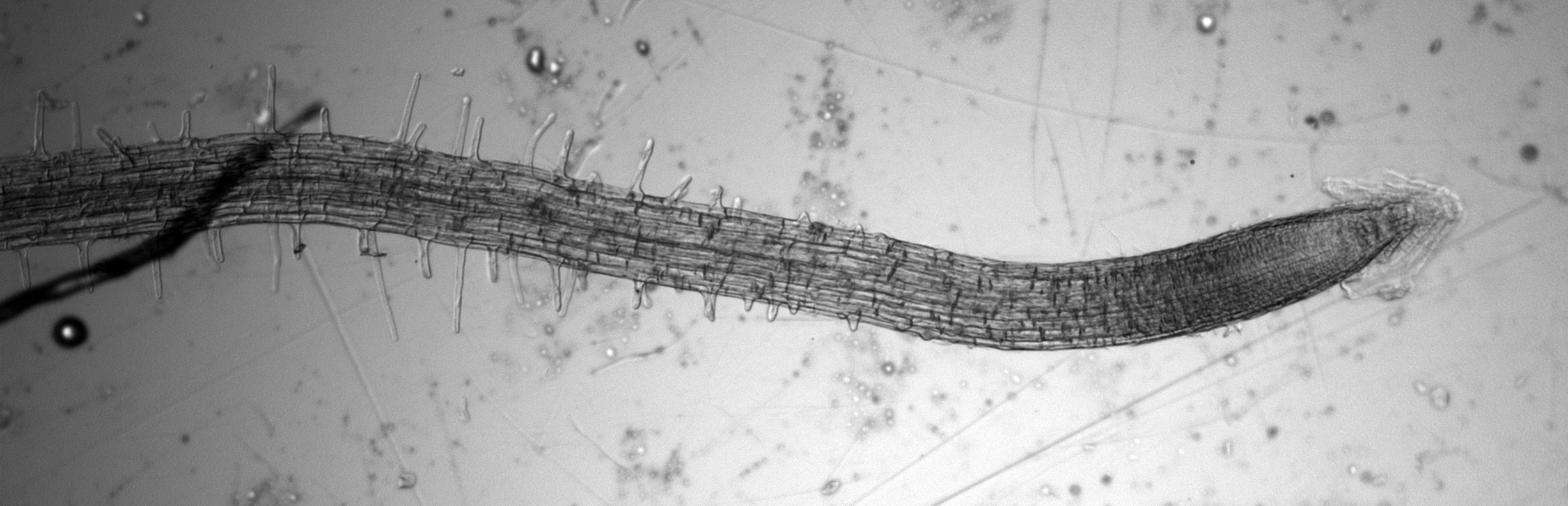
But some progress happened on the root growth project. Having decided that I could make some hay using good old transmitted light (i.e., bright-field) microscopy, I made some movies. The unit here has a sweet little compound microscope that can rest solidly on its back. The stage has also been modified to hold a square Petri plate, on which grow the lab weed seedlings. A high-resolution camera is available for imaging and a no-frills piece of software to control the camera and grab images. There are ten-X and five-X objectives, to give a modest magnification. An image of the root looks like this:
Lab weed root surrounded by water, the usual type of image for roots growing on agar medium
I have a set-up rather similar to this back at Amherst. In fact, it has been well used to study root growth. But in all of those experiments, the analysis has been for a single moment in time. A snapshot as it were of the growth status of that particular root. And the questions asked have all been based on comparing different groups of roots; for example, what is the effect of some inhibitor on the pattern of growth.
What I am interested in doing here is to look at the same root over time. How does the pattern of growth within the root change over time? In the end, I want to address this question with cellular resolution and that is why I am ultimately going to be working with the roots with fluorescent cell walls. But to get that data, I need new software, which I hope will be written before long, but isn’t written yet. I realized that I can use the software I already have to gain some information about how the growth pattern changes over time. Not at cellular resolution but useful all the same. This is what I have started to do.
In theory, it is quite straightforward: get the root in front of the microscope, image as shown above and capture images for an hour or so and then analyze the growth at many times during the hour. Now, look again at the picture of the root above. Look at the thick black zone around the root. This black area is actually a film of water that surrounds the root. This is a feature of roots growing on agar—the water wicks up around them. The water obscures the edges of the root, cutting down on the useful information available in the image. One work-around is to use higher magnification. This doesn’t change the black side-band, but allows the inner, useful region of the root to span more pixels and hence be analyzed for growth at greater resolution. The downside of higher magnification is that the growth zone can no longer be imaged in one field of view.
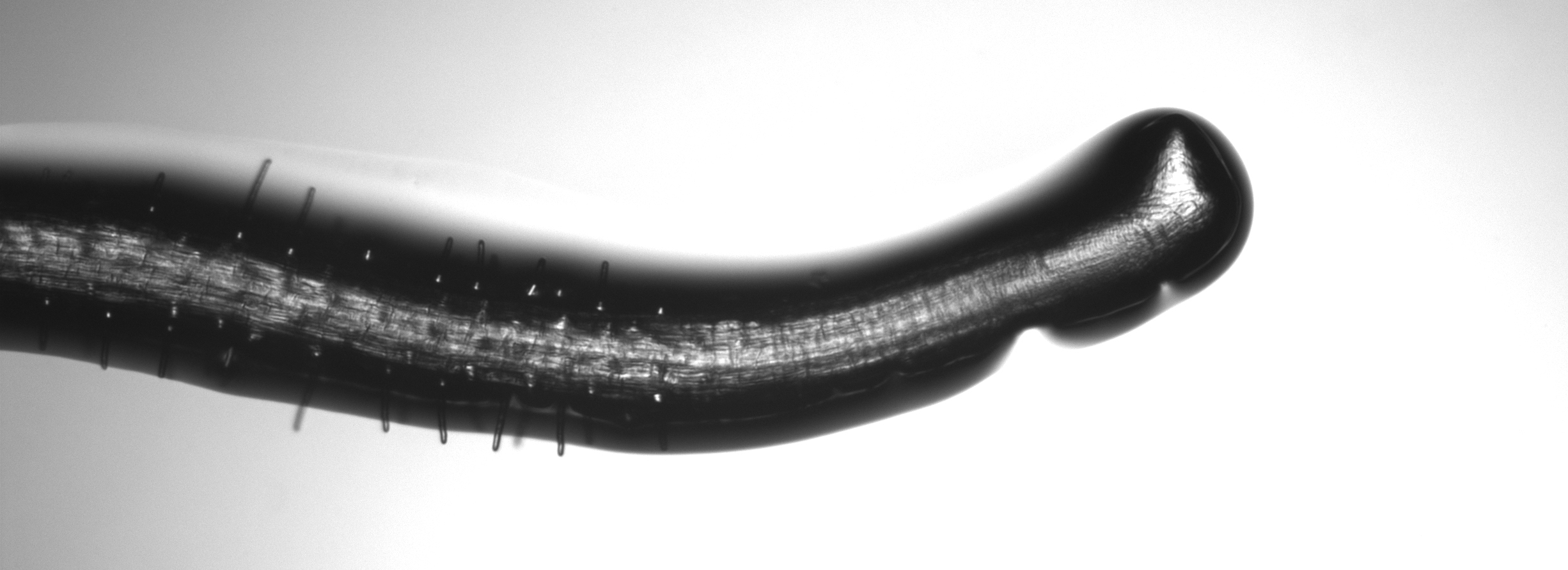
The folks at CPIB have their hands on another potential work-around. They have found a thin cellophane-like film that is gas permeable and available for sale. One puts a small square of the film right on top of the root. The effect is rather like putting a coverslip on, removing the optical interference from the water film. But in contrast to a glass coverslip, this special film permits those precious oxygen molecules to enter. A root with this film on looks like this:
Lab weed root under a gas permeable film
Now, the root is imaged clearly, right out to the very edge. On the other hand, there is always one of those other hands–sometimes ten of them, the film is prone to accumulating dust. That explains all those background spots and junk in the image. There was so much of that gunk on one of the roots that there was no point in imaging it.
Anyway, I took movies of roots, both with and without film. Some at 10-X and some at 5-X. Each of the movies are more correctly termed ‘image sequences’. That is, I acquire an image of the root at some fixed time interval, this week the interval was one minute. The images can be played back like a movie, one sees the root growing, but for analysis purposes, I will analyze pairs of images. Because it is easier to type ‘movie’ than ‘image sequence’, I’ll use the former, unless I am feeling punctilious.
And then the analysis. To do this, I will use software written in my lab called ‘stripflow’. This software runs in a powerful package called “Matlab”. I have used Matlab once or twice and I have helped various students and collaborators use stripflow, but I have limited experience with my own hands. One job this week was firing up Matlab and running the stripflow code and remembering how it all works. There were some hiccups and glitches. But in the end, I could produce a picture like this:
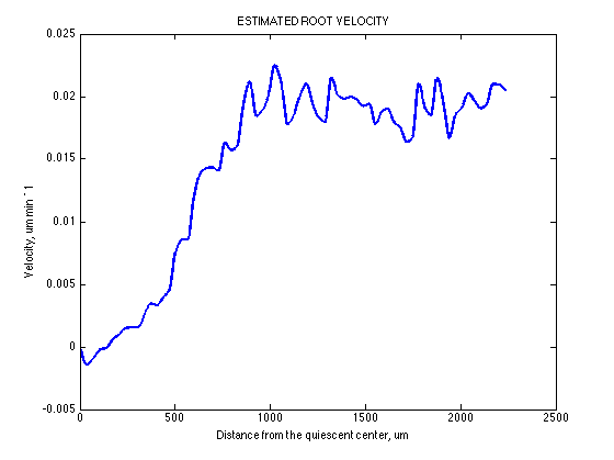
Velocity profile of a growing root
This is a plot of velocity versus distance. It represents the velocity (the movement) that occurred over the one minute between images. But what is this plot all about?
Let’s start with the x-axis: “distance from the quiescent center”. The latter is botanical verbiage for a point-like region at the tip of the root (just four cells in lab weed). There are reasons for using this point, rather than very apex of root but for thinking about this plot it is fine to think about the x-axis as representing distance from the tip.
With the x-axis taken care of, let’s cope with the y. The plotted velocity shows how fast a point at each distance from the root tip is moving. We know that the tip of root moves down as the root grows. If we wanted to measure the rate of “root growth” we would measure the rate at which the root tip progresses downward. This rate is a velocity. Having said that, it should puzzle you that, in the plot above, the velocity at the root tip is zero. Hmmm. The resolution is that here the data are plotted with respect to the root tip. Imagine sitting right on the root tip, moving with root tip. You would feel motionless and the mature part of the root base would seem to be moving away from you (like sitting on a moving train). The mature regions the root would be moving away from you at exactly the rate of “root growth” (i.e., at the rate at which the tip moves past the motionless soil). That is why the velocity from about 700 microns to the end of the graph is constant (at about 0.018 microns per min—actually that is a typo in the y-axis, it should be microns per sec).
Why do we care about velocity anyway? We care because it embodies the growth of local (i.e., sub-cellular) regions. Think of it this way: If a region and its neighbor have the same velocity, there is no growth between them; whereas, if one region moves faster than its neighbor, there *is* growth between them. In fact, this description can be inverted to say that the reason there is velocity to measure is because the root is growing. Enlargement causes movement.
Now that I could coax stripflow to cough up a velocity profile, my task is to generate velocity profiles for the movies, perhaps every minute, perhaps less frequently, and look at how that profile changes. I started to do that and to work out a couple of issues related to optimizing and streamlining the task, because that is a lot of profiles and so streamlining would be good thing. But first, there is a nastier problem that needs to be mentioned and I need to figure out how to overcome.
I noticed this when I was imaging, and the plots (like the above) confirmed, these film-star roots were growing slowly. Very slowly. That maximum velocity I mentioned a moment ago is about four or five times slower than I was expecting. Furthermore, when finished with the movies, I marked the position of the root tips on the two plates I was working with (about two dozen roots all told), and the next day, the roots had not grown an iota. This is extremely odd. It suggests that somehow the plates were problematic. Or maybe the plants. This is the atrocity I referred to hyperbolically in the title of the post.
I had just scrounged those plates. Usually one makes plates in sets of twenty or forty but I just need one or two, and people were generous in letting me take a couple. Like bumming cigarettes. Maybe I got a menthol flavored one? I decided that I had best be on top of my plates, know what is in them and no surprises. Therefore, this week, I made plates. Haven’t done that in years! This is like cooking where you add so much of this and so much of that and then autoclave it, so that no bacteria or fungi keep the lab weed company. The autoclave also dissolves the agar powder. Well, besides adding 10-times too little agar and sucrose (but I caught that before it was too late) and besides pouring agar on top of the lid of a plate instead of inside it (a minor mess), it went fine. I planted seeds on them, so the next round of movies can with any luck be taken on plants growing properly. Nice well behaved Victorian proper plants!
delightful blog Tobais!
Has anyone done what you are doing in the expanding young cereal leaf, which exapnds in essentially the same way as your root with different parts expanding at different rates and the basal meristem giving rise to new cells. Its the same as your root but the other end is attached!
cheers
kevin
Kevin,
Thanks! Certainly, kinematic analyses of cereal leaves have been done, maybe even more than for dicot leaves, for exactly the reason you say. There is work by Curtis Nelson and students, Francois Tardieu, and others. But the tricky bit here is that the growing part of the leaf is sheathed by older non growing parts of leaves. So marks have been applied by using pinpricks. This gives a snapshot of the growth profile. And valuably so. But I aim here to follow the growth profile as it changes over time. This would require a whole lot of pricking. Perhaps when CT power unleashed at Houndsfield, this can become practical???