6.3 Command group ANALYSIS |
The Analysis command group contains several tools for image analysis in real space as well as in Fourier space. Furthermore you can fit the parameters for the PCTF (Phase Contrast Transfer Function) and combine an image out of tiles.
There are two buttons side by side to deal with the Fourier analysis: ![]()
![]() With the left button the powerspectrum of the actual image is calculated and displayed. The right button opens a little popup menu where you find some special scaling functions for powerspectra.
With the left button the powerspectrum of the actual image is calculated and displayed. The right button opens a little popup menu where you find some special scaling functions for powerspectra.
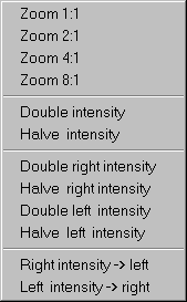 |
The first group contains four instructions to set the zoomfactor on the center of the powerspectrum.
The two instructions in the second group change the overall intensity of the displayed powerspectrum.
In the third group you can alter the intensity of either the right or the left half of the powerspectrum.
With the instructions in the last group, the intensities of one half is also used for the other half.
The 'Linescan' starts after pressing ![]() in 'Histogram' mode.
in 'Histogram' mode.
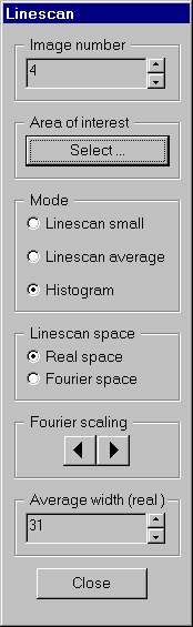  |
The 'Linecsan' is designed for pixel operations on stored or acquired images and provides the following functions:
For convenient comparison of the same subareas of different images of an image series, you can change the current image and viewportnumber in the section 'Image number'.
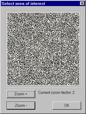
Select a square subarea of the image in the 'Area of interest' section:
 |
In the 'Mode' group you can chose one of three modes:
Using Ctrl(Strg) key or Shift key while moving the line in real space mode, the line will automatically be converted into a vertical or horicontal line, respectively.
In all mode/space combinations the plot can be modified with the buttons
![]() or
or ![]() .
The plot is updated immediately.
A click on
.
The plot is updated immediately.
A click on
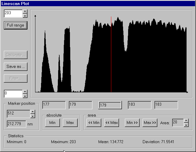
![]() displays the full data range.
displays the full data range.
Within the plot dialog you can move the current-value-marker either with a click in the plot area, or ( e.g. for fine positioning ) using the spin control
in the section 'Marker position'. The field below the plot with the fat border shows the value direcly under the marker, the 2 fields to the left and right
show the values next to the marker ( if available ). Another possibility to move the marker are the Min/Max buttons. Clicking on ![]() in the
section 'absolute' the marker is positioned on the absolute minimum or maximum, respectively, of the whole plot.
Clicking on one of the 4 buttons
in the
section 'absolute' the marker is positioned on the absolute minimum or maximum, respectively, of the whole plot.
Clicking on one of the 4 buttons ![]() moves the marker to the next minimum or maximum
in the desired direction. The minimum/maximum search is restricted to the specified area. If e.g. Area is set to 20 and
moves the marker to the next minimum or maximum
in the desired direction. The minimum/maximum search is restricted to the specified area. If e.g. Area is set to 20 and
![]() is clicked,
the marker is positioned on the maximal plot value in the area [current position-20 .. current position-1].
If you are in linescan real or linescan fourier mode you have also the possibility to move the marker within the image.
is clicked,
the marker is positioned on the maximal plot value in the area [current position-20 .. current position-1].
If you are in linescan real or linescan fourier mode you have also the possibility to move the marker within the image.
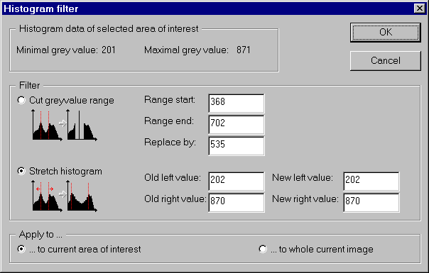 |
If you are in the histogram mode, the button ![]() in the histogram plot dialog will be enabled.
A click on this button opens the histogram filter dialog
that provides 2 histogram filters. Both filters will change the image data ! 'Cut greyvalue range' filter will replace all the occurrences
of the greyvalues within the range specified by 'Range start' and 'Range end' by the greyvalue specified in 'Replace by'.
'Stretch histogram' squeezes or stretches the histogram. The data between the left start point and 'Old left value' are rescaled to the area left
start point and 'New left value'. The data between 'Old left value' and 'Old right value' are rescaled between 'New left value' and 'New right value' and
finally the data between 'Old right value' and the most right position are rescaled between 'New right value' and the most right position. Those filters
can be applied either to the whole image or the current area of interest.
in the histogram plot dialog will be enabled.
A click on this button opens the histogram filter dialog
that provides 2 histogram filters. Both filters will change the image data ! 'Cut greyvalue range' filter will replace all the occurrences
of the greyvalues within the range specified by 'Range start' and 'Range end' by the greyvalue specified in 'Replace by'.
'Stretch histogram' squeezes or stretches the histogram. The data between the left start point and 'Old left value' are rescaled to the area left
start point and 'New left value'. The data between 'Old left value' and 'Old right value' are rescaled between 'New left value' and 'New right value' and
finally the data between 'Old right value' and the most right position are rescaled between 'New right value' and the most right position. Those filters
can be applied either to the whole image or the current area of interest.
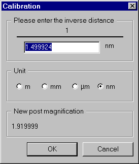 |
You can calibrate the postmagnification ( and hereby also the distance in real space ) by clicking on the button ![]() in the linescan plot
dialog. This button is only enabled for the linescan fourier mode. For the calibration you need an image of a crystal with well-known properties. Adjust
the linscan in such a way that a typical reflex is seen in the plot. Move the marker exactly over this reflex ( a peak in the plot ) and click
in the linescan plot
dialog. This button is only enabled for the linescan fourier mode. For the calibration you need an image of a crystal with well-known properties. Adjust
the linscan in such a way that a typical reflex is seen in the plot. Move the marker exactly over this reflex ( a peak in the plot ) and click ![]() .
In the calibration dialog enter the inverse distance of that reflex in the edit field and you will see the new post magnification. This value has to be entered
in the mag.conf file for the current magnification.
.
In the calibration dialog enter the inverse distance of that reflex in the edit field and you will see the new post magnification. This value has to be entered
in the mag.conf file for the current magnification.
To save the plot data into an ASCII file, click on ![]() and a file selector dialog will open. Select the
directory and filename you like and the plot data is written into this file.
and a file selector dialog will open. Select the
directory and filename you like and the plot data is written into this file.
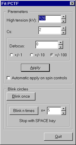
If you have a suitable powerspectrum, you can use this to check/fit the parameters HT (= High Tension), Cs (= spherical aberration) and Dz (= defocus). Start this dialog with ![]() .
.
 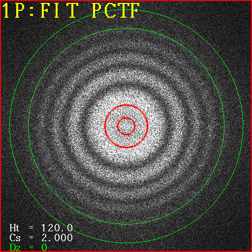 |
In the lower left corner of the display are the actual values for the hightension, the spherical aberration and the defocus displayed. The green circles in the powerspectrum represent the positions of the minima in the powerspectrum as they are calculated with the given parameters.
In the "Fit PCTF" page you can now change the parameters, and the position of the green circles are recalculated either immediately with every change (if the checkbox 'Automatic apply on spin controls' is activated) or after pressing ![]() button.
button.
As a little help for comparing the position of the green circles with the minima in the powerspectrum you can let the circles blink once or n times.
Hint: if you want to stop blinking circles with the <SPACE> key just type it once. A second strike just starts the blink cycle again!
The 'Fourier filter' dialog makes various filter operations in spacial space available:
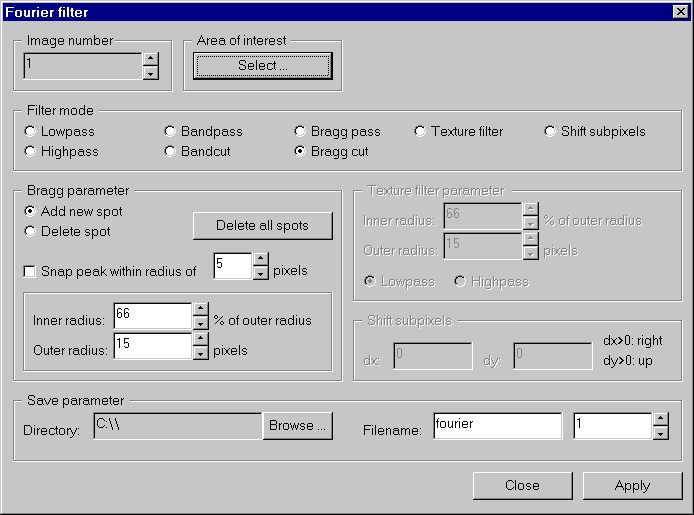 |
When the 'Fourier filter' dialog is started, the power spectrum of the actual image is calculated and displayed in the actual viewport. You can now select another image number and/or an area of interest.
Select now the desired filter function and enter the parameters belonging to this filter. For the Bragg filters, the texture filter and the shift subpixel method the parameters are entered within the 'Fourier filter' dialog. For the other parameters use the green selection rings on the display:
 |
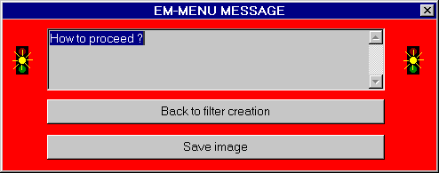
Once you have applied the filter, you are asked how to proceed:
 |
In the 'Save parameter' section is determined where the results are stored.
If you have an image series with overlapping images, you can use the 'Tiling' dialog to fit the images to one
single image. Invoke the 'Tiling' dialog with ![]() .
.
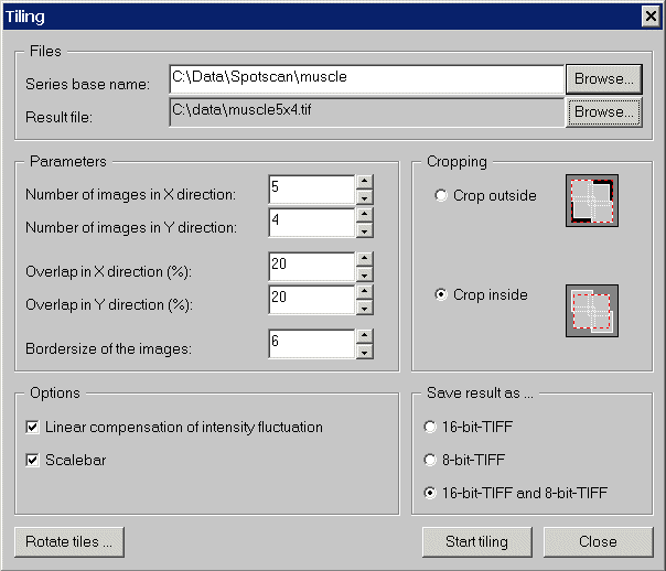 |
The tiling algorithm will combine a set of images into one big image. It is assumed that the images in the series are stored on a row by row base. It is necessary that the images have overlapping areas and that the size of those overlapping areas ( in percent ) is entered as exact as possible. Otherwise the tiling will fail.
In the section Files you can either enter directly or browse for the path plus the basename of the image series you want
to combine to one image. If e.g. the files muscle_001.dat, muscle_002.dat, ... of the directory C:\Data\Spotscan shall be used,
this field must contain: C:\Data\Spotscan\muscle .
Additionally you have to specify the path and filename of the result image.
In the section Parameters you have to specify the number of images in x and y direction, as well as the estimated overlap in
both directions.
Additionally you have to specify the size of the borders the images might have.
In the section Cropping you can select between cropping outside and cropping inside. In most cases the images do not fit exactly in x
and y direction, i.e. the resulting image will not have continuous borders. If crop outside is selected, all the tiled image data will be
found in the resulting image and the undefined areas will be filled with black.
If crop inside is selected, the image will be clipped to the maximal rectangle that fits into the tiled image.
In the section Options you can disable/enable Linear compensation of intensity fluctuation and Scalebar.
If Linear compensation of intensity fluctuation is selected, the overlapping areas of the images are analyzed and the corresponding images are multiplied
by a correction factor to reduce illumination differences that occurred during image acquisition.
If Scalebar is selected, a scalebar will be copied into the upper left corner of the image.
In the section Save as you can select whether the image data is stored in 16 bit TIF format, in 8 bit TIF format or both. The result is written into the file specified in result file, except if both formats are desired. In that case, the 16 bit image is stored in the specified file and the 8 bit image is stored in a file with the same path, but the filename is extended by _8bit, e.g. result.tif (for the 16 bit data image) and result_8bit.tif (for the 8 bit data image).
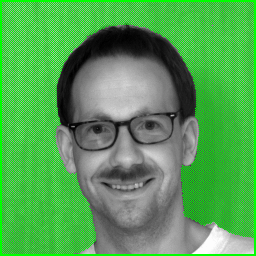
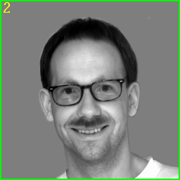
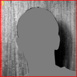
This analysis tool enables you to select/remove specific areas of an image for detailed analysis. You can e.g. remove undesired parts of an image, or specify areas of interest, or ... . A click on Mask ... in the main dialog displays the current image covered completely with a green mask:
 |
The left mouse button controls the drawing/removing of the mask, whereas the right mouse button opens a popup menu. To clear the mask with the current pencil, hold the shift key pressed, while moving the mouse with the left mouse button pressed. To set the mask at a specified position, hold the ctrl-key, while moving the mouse with the left mouse button pressed. If you move the mouse with the left mouse button pressed but without pressing any key, the currently selected mode ( add to mask / remove from mask ) will be applied. The mouse cursor indicates the operation. A plus sign indicates "adding to the mask" while a minus sign means "removing from the mask".
| Mouse cursor for adding mask | |
| Mouse cursor for removing mask |
A klick on the right mouse button opens a popup menu:
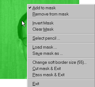 |
The menu items have the following meaning:
| Add to mask | When pressing the left mouse button without shift or ctrl key, an area of the current pencil is added to the mask at the current mouse position |
| Remove from mask | When pressing the left mouse button without shift or ctrl key, an area of the current pencil is removed from the mask at the current mouse position |
| Invert mask | Inverts the current mask |
| Clear mask | Clears the current mask |
| Select pencil ... | Opens a dialog where you can select a pencil ( see below ) |
| Load mask ... | Loads a mask from a file. The windows open file dialog opens and you have to specify the file with the mask in it. |
| Save mask as ... | Saves a mask to file. The windows save file dialog opens and you have to specify the filename and path of the file you want to store the mask in. |
| Change soft boder size (nn) | When applying the mask to the image optionally the border can be softened. Therefore an area of nn by nn pixels is analyzed. (nn) shows the currently selected value. To change this value select this menu item and a dialog opens where you can select a new value. |
| Cut mask & Exit | Apply the mask to the image. All pixels covered by the mask will be replaced by the mean value of all unmasked pixels. Then the mask creation is terminated and the resulting image displayed. |
| Pass mask & Exit | Apply the mask to the image. All pixels covered by the mask will held, all other pixels will be replaced by the mean value of all masked pixels. Then the mask creation is terminated and the resulting image displayed. |
| Exit | Exit mask creation without applying it to the image. |
Example:
Have a look at the following images. The left one is the image with the mask, the middle one was created using Cut mask & Exit and the right one using Pass mask & Exit
 |
 |
 |
To select different pencils, click with the right mouse button and in the popup menu select the menu item Select pencil... .
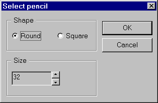 |
There are 2 types of pencils available: Round ones and square ones. Select the shape using the corresponding radio button. Select the size of the pencil using the spin control.
Note: The size of the pencil is in image coordinates. I.e if you edit a 512x512 image in a 512x512 viewport and use a pencil of 32x32 pixel, then there will be a 32x32 pixel pencil visible in the display. If you however edit a 2048x2048 image within a 256x256 viewport, a 32x32 pencil will be nearly invisible, since for display purposes it will be reduced by factor 8x8, i.e. a 4x4 pencil will be visible. Note that this reduction is only for display, a 32x32 pencil is nevertheless applied to the mask .
After a click on ![]() the statistics of the current image and of subimages of the current image are computed
and displayed:
the statistics of the current image and of subimages of the current image are computed
and displayed:
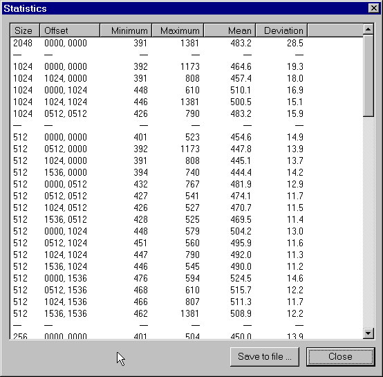 |
Of a n*n image the following (sub)images are computed:
The minimum, maximum, mean and root mean square deviation are displayed for each of that subimages together with the size and the offset ( relative to the upper left corner).
Last update: